Introduction
I recently released the initial version of the Simulation Catalogue. Along with it came the charged particle in a magnetic field simulation, which calculates the trajectory of a charged particle moving in a constant magnetic, electric, and gravitational field (more on that here).
Despite positive initial results, a closer inspection of the results revealed some issues.
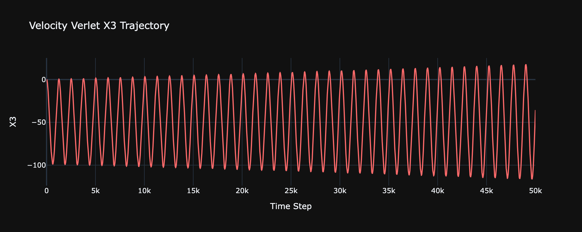
x3 evolution showing instability in x3 plane.
At first glance this looks exactly as expected. The magnetic field is causing the charged particle to oscillate in the plane. However, a closer look shows that the amplitude of the oscillation is increasing over time, ultimately resulting in an unstable trajectory.
A Closer Look at Velocity Verlet
Unstable trajectories usually point to an issue with the underlying algorithm. In this case, I was using Velocity Verlet, a common "leapfrog" style algorithm used to model a whole host of physical systems with great success.
Velocity Verlet updates the velocity of the particle in half-steps, and is implemented in the following manner:
- Calculate
- Calculate
- Calculate
where the acceleration is re-computed between each velocity update.
Usually, the result is a sort of self-stabilizing trajectory. Instabilities do occur, but they self-regulate over the course of the simulation. The particle may veer off its trajectory slightly in one iteration of the loop, but it will veer off in the opposite direction in a subsequent iteration. Errors average themselves out.
However, this clearly isn't happening here. So what's going on? The answer is that Velocity Verlet does not work with velocity dependent forces. Step 3 involves computing the force at . However, this requires knowing . If the force depends on the velocity, a circular definition is introduced. The only way to compute the force is to use the velocity at , which is incorrect. This is the source of the instability.
It's worth mentioning here that the initial Velocity Verlet implementation did produce sensible results, especially in cases where the time step is small and the initial conditions are relatively stable.
Solving the instability required a more sophisticated algorithm that handled the velocity dependence explicitly. This is where the Boris Pusher comes into play.
The Boris Pusher Algorithm
Handling the velocity dependence requires a more subtle approach. The Boris Pusher is the gold standard when it comes to plasma physics simulations. It separates forces into two separate batches: those that cause linear acceleration (electric fields, gravity etc) and those that cause gyration of the velocity vector (magnetic) field.
- Use linear forces to compute the first half-kicked velocity vector
- Rotate the half-kicked velocity vector using the magnetic field
- Use linear forces to compute the second half-kicked velocity vector
- Calculate final position
Mathematically, this can be broken down into the following
There's an important caveat here: the Boris Pusher implemented this way only works because the fields (electric, magnetic and gravitational) are constant i.e they do not depend on the position of the particle. This allows us to compute the final velocity and position updates at the very end.
The Boris Pusher can be used for non-constant fields as well. One easy approach is to simply evaluate the fields before the Boris Push is started using the current position vector. This is often good enough for fields that vary slowly relative to the gyration radius. Another slightly more accurate approach is to estimate the half step position and use that to evaluate the fields.
Implementation
With the algorithm in place, it's time to write the Fortran implementation. Since this was the second integrator that I wrote, I decided to implement a generic integrator interface. This allows me to define a whole series of integrators that I can use interchangeably throughout the codebase.
module integrators
  implicit none
  private

  type, abstract, public :: integrator_t
    real :: delta_t

  contains
    procedure(step_proto), deferred, pass(this) :: integrate_step

  end type integrator_t

  abstract interface
      subroutine step_proto(this, particle, force)
         import integrator_t
         import PointParticle
         import force_t

         class(integrator_t), intent(in) :: this  !< The integrator instance
         type(PointParticle), intent(inout) :: particle  !< Particle to update
         class(force_t) :: force  !< Force calculator
      end subroutine step_proto
  end interface
end module integrators
Lets quickly break down whats going on here. First I define a integrator_t abstract type, which has a integrate_step procedure attached. integrate_step must implement the proto_step abstract interface. Think of it this way: integrator_t is the integrator, integrate_step defines how the integrator performs numerical integration.
Note that integrate_step relies on a few custom types that are defined in other modules, mainly PointParticle and force_t. I won't cover these in detail here, but PointParticle is a type that holds the basic properties (mass, charge etc) and mechanical state (velocity, position etc) for a point particle. force_t is another abstract type that has a get_force function which generates the force vector acting on a given PointParticle instance.
With the interface in place, the Boris implementation can be created.
module integrators
  type, extends(integrator_t), public :: boris_t
    real, dimension(3) :: magnetic_field

  contains
    procedure, pass(this) :: integrate_step => boris_step

  end type boris_t

contains
  subroutine boris_step(this, particle, force)
    class(boris_t), intent(in) :: this
    type(PointParticle), intent(inout) :: particle
    class(force_t), intent(in) :: force

    real :: a_linear(3)
    real :: v_minus(3), v_prime(3), v_plus(3), t_vector(3), s_vector(3)

    ! calculate force due to linear components
    a_linear = force%get_force(particle)/particle%mass
    ! do first velocity update
    v_minus = particle%state%velocity + a_linear*(this%delta_t/2)

    ! define tangent and secant vectors
    t_vector = (particle%charge/particle%mass)*this%magnetic_field*(this%delta_t/2)
    s_vector = (2*t_vector)/(1 + dot_product(t_vector, t_vector))

    v_prime = v_minus + cross_product(v_minus, t_vector)
    v_plus = v_minus + cross_product(v_prime, s_vector)

    particle%state%velocity = v_plus + a_linear*(this%delta_t/2)
    particle%state%position = particle%state%position + particle%state%velocity*this%delta_t

  end subroutine boris_step

  function new_boris_integrator(delta_t, magnetic_field) result(integrator)
    real, intent(in) :: delta_t
    real, intent(in) :: magnetic_field(3)
    type(boris_t) :: integrator

    integrator%delta_t = delta_t
    integrator%magnetic_field = magnetic_field

   end function new_boris_integrator

end module integrators
boris_t is defined as a type that extends our integrator_t interface. The magnetic field is also set as an attribute of the boris_t type. Next we define a subroutine called boris_step which implements the algorithm outlined above. Note that the signature of the subroutine must match precisely that of the proto_step abstract interface, otherwise the code won't compile. Finally, the boris_step subroutine is attached to the boris_t type as its implementation of proto_step.
All thats left is to replace the old verlet velocity code with the new boris step integrator
program boris_example
  use integrators
  implicit none

  type(boris_t) :: boris_integrator
  type(lorentz_force_t) :: force
  type(PointParticle) :: particle

  real, dimension(3) :: magnetic_field, electric_field
  real, dimension(3) :: initial_position, initial_velocity
  real :: charge, mass
  real, dimension(:, :), allocatable :: trajectory
  real :: delta_t
  integer :: num_steps, i

  delta_t = 0.01
  num_steps = 5000

  charge = 1.0
  mass = 1.0

  magnetic_field = [1.0, 0.0, 0.0]
  electric_field = [0.0, 2.0, 1.0]

  initial_position = [0.0, 0.0, 0.0]
  initial_velocity = [1.0, 5.0, 5.0]

  ! define force acting on particle
  force = new_lorentz_force_t(electric_field, magnetic_field)

  allocate(trajectory(num_steps, 3))
  ! create new boris integrator
  boris_integrator = new_boris_integrator(delta_t, magnetic_field)

  ! create new point particle instance
  particle = new_point_particle(mass, charge, initial_position, initial_velocity)

  do i = 1, num_steps
    ! call the integrate_step() subroutine with each iteration
    call boris_integrator%integrate_step(particle, force)
    ! update the trajectory
    trajectory(i, :) = particle%state%position
  end do

end program
Hopefully now it becomes clear why I went to the trouble of defining the abstract type integrator_t. I can now swap out the boris_t integrator for any other type that implements integrator_t without changing the rest of the code.
Results
Now comes the relevant part. It's all for nothing if it doesn't stabilize the trajectory. The following simulation configuration was used to test the new Boris implementation.
[parameters]
initial_velocity = [1.0, 5.0, 1.0]
initial_position = [0.0, 0.0, 0.0]
magnetic_field = [0.25, 0.0, 0.0]
electric_field = [0.0, 0.0, 0.0]
mass = 0.25
charge = 0.5
delta_t = 0.01
num_steps = 50000

[config]
output_dir = "output"
The following figure shows the individual trajectory components for both the verlet and the boris algorithm.
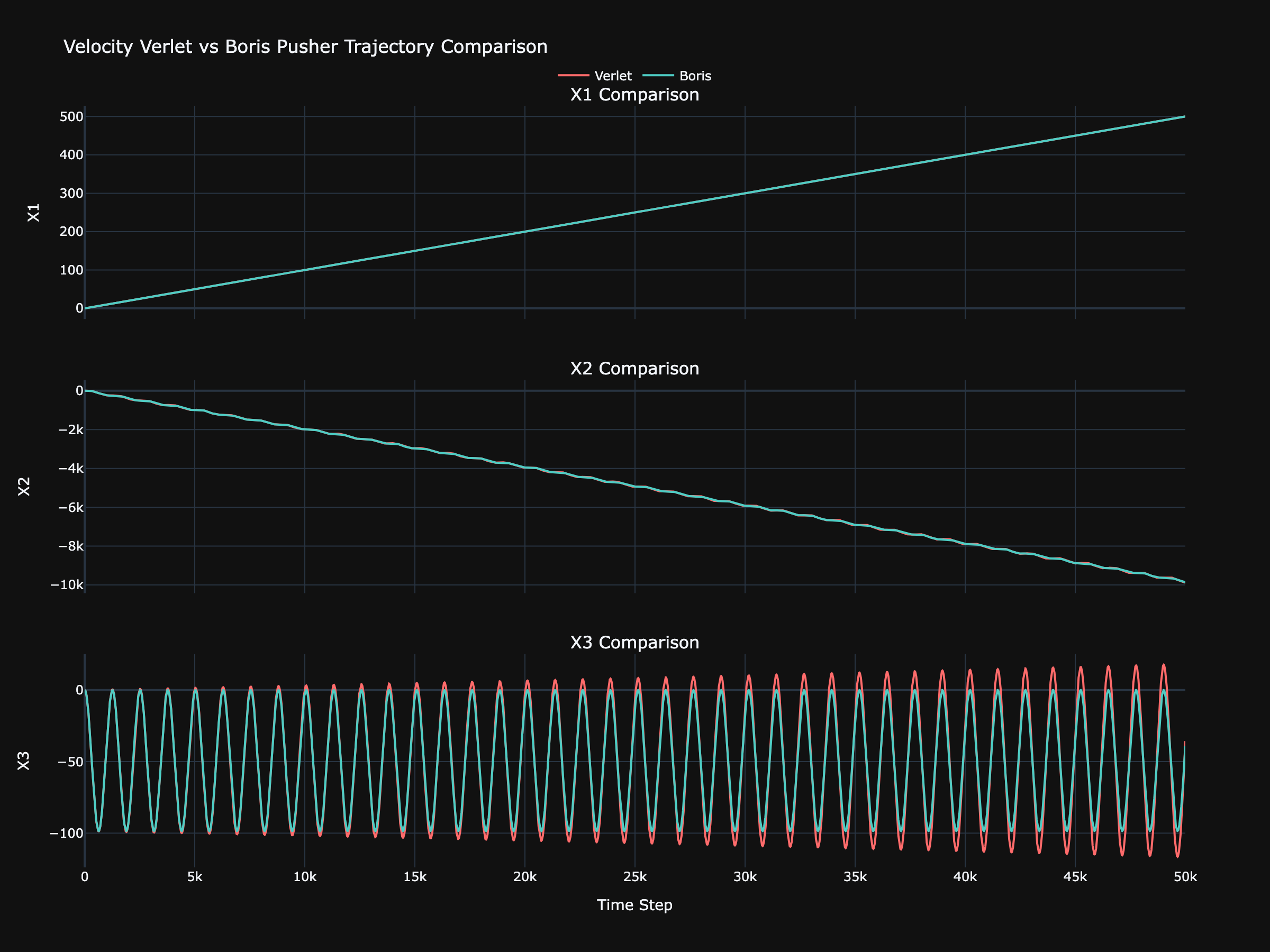
Trajectory for Verlet and Boris Algorithm.
The evolution in and was largely unchanged. Closer inspection of does reveal a slightly more stable trajectory. The Verlet algorithm doesn't break down quite as much in as it does in , but the Boris implementation does produce a smoother path.
The difference in the component however is drastic. Much like before, the Verlet algorithm almost instantly produces an unstable trajectory. The Boris algorithm on the other hand, is completely stable.
Outcomes and Learnings
It will come as little surprise to anyone with expertise in the field that the Boris Pusher Algorithm outperforms Velocity Verlet on every metric. It's definitely a useful tool, and will likely become my de facto algorithm for future simulations that involve magnetic fields.
The abstract type approach used in the Fortran code for the integrators and forces proved to be useful as well. I was able to run the simulation with the Boris and Verlet algorithms almost interchangeably to produce the plots for analysis, with very little code changes between iterations.
There are definitely improvements to be made, especially to the force_t interface, which really needs to be revised to encapsulate a field rather than a single force. Updating the Boris implementation to handle time and position dependent fields is also a natural evolution of the current code, and will be required for more complicated systems.
But overall, I achieved what I set out to do. The Boris algorithm stabilized the trajectory, which not only produced better plots, but also drastically saves me on compute. I was able to reduce both the time step and the number of iterations by an order of magnitude in the live simulation catalogue. The simulation runs 10x faster, and produces better results. A definite success.
Some of the code provided in this article was a little rushed. If you're interested in seeing the implementation thats actually running on this platform, feel free to visit the GitHub repo.